Chapter 3 Probability and Counting
Probability is a tricky subject. We have an intuitive sense about probability, but we use it in different ways, which can sometimes lead to confusion. Probability is used in at least two ways:
-to describe the relative frequency of events, e.g., what is the chance of observing 5 heads in the next ten flips of a fair coin; and,
-to communicate degrees of belief, e.g., the Packers have a 30% chance of winning the Super Bowl.
We will use probability exclusively in the sense of the first interpretation—to characterize the chances of different outcomes in repeatable trials. This sense of probability corresponds to characterizing the possible outcomes of random sampling. Although probability is often used to communicate degrees of belief there are good reasons not to use it for this purpose, but a formal, nuanced discussion of quantification of beliefs is outside our present purview.
3.1 Terminology
In our discussion of probability we will think of an experiment as the act of measuring/observing a variable on one or more random samples from a population. The sample space is the set of possible realizations of the experiment. For example, if the experiment is to flip one coin and record whether it is heads or tails, then we can think of this as a random sampling from sample space \(\{H, T\}\) where the outcome may be either \(\{H\}\) or \(\{T\}\). Any subset of the sample space of an experiment is an event; for example, \(\{H\}\) and \(\{H,T\}\) are events, and so is \(\emptyset\) which denotes the “empty set,” the set of nothing.
3.2 Set relations
Events and sample spaces are sets, and we will make use of relations between sets.
-Set union: for sets/events A and B, \(A\cup B\) denotes the set of elements in at least one of \(A\) or \(B\). For example, \(\{1,2,3\}\cup\{3,4,5\} = \{1,2,3,4,5\}\).
-Set intersection: \(A\cap B\) denotes the set of elements in both A and B. For example, \(\{1,2,3\}\cap\{3,4,5\} = \{3\}\).
-Set complement: \(A^c\) denotes the set of elements in the sample space \(\mathcal{S}\) but not in \(A\). For example, if \(\mathcal{S} = \{1,2,3,4,5\}\) then \(A^c = \{4,5\}\).
-Set subtraction: \(A\backslash B\) of \(A-B\) means \(A\cap B^c\) which is the set of elements in \(A\) but not in \(B\). For example, \(\{1,2,3\}-\{3,4,5\} = \{1,2\}\).
3.2.1 Sample space example
Here’s an example to illustrate sample spaces. A gas station has six pumps, A, B, C, D, E, F.
-What is the sample space of the number of pumps in use? \(\mathcal{S} =\{0,1,2,3,4,5,6\}\).
-What is the sample space of pumps in use? \(\mathcal{S} = \{\{A,B,C,D,E,F\},\{A,B,C,D,E\}, \ldots,\{F\}, \emptyset \}\). This is the power set of \(\{A,B,C,D,E,F\}\), the set of all subsets of those pumps. Fun fact: if the sample space \(\mathcal{S}\) consists of \(N\) elements then its power set, written \(2^{\mathcal{S}}\), contains \(2^N\) elements. Can you see why?
-Suppose you test pump A every day until it fails to function. What is the sample space of this experiment? \(\mathcal{S} = \{F, SF, SSF, \ldots \}\). This is a countably infinite sample space.
-You measure the amount of gas pumped by the next customer. \(\mathcal{S} = (0, ?)\), an interval with some upper bound equal to however much gas the station has available. This is an uncountably infinite sample space.
3.2.2 Set relations example
This next example illustrates set relations.
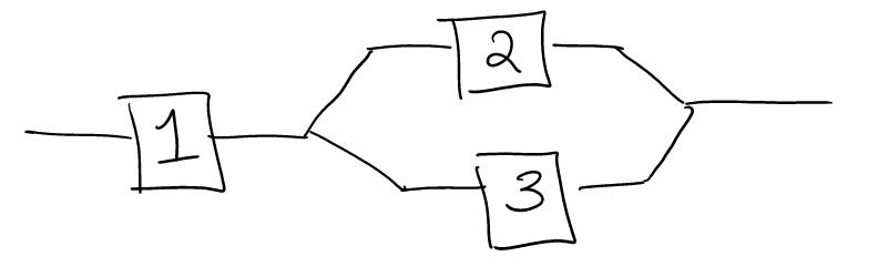 Consider this system of series and parallel components. Each component either functions/succeeds (S) or fails (F). The experiment simply observes if the system functions/succeeds or fails.
-What is the sample space in terms of the three components? \(\mathcal{S} = \{SSS, SSF, SFS, FSS, SFF, FFS, FSF, FFF\}\).
-Find the even two components succeed. \(A = \{SSF, SFS, FSS\}\).
-Find the even at leas two components succeed. \(B = \{SSF, SFS, FSS, SSS\} = A\cup \{SSS\}\).
-Find the event the system functions. \(C = \{SSS, SFS, SSF\}\).
3.3 Probability Axioms
Andrey Kolmogorov formalized rules/axioms of probability we are mostly, intuitively familiar with.
- The probability of the sample space is 1, \(P(\mathcal{S})=1\).
- Probabilities are non-negative. If \(A\subset\mathcal{S}\) then \(P(A)\geq 0\).
- Countable additivity. This last one is a bit tricky. Let’s start with an intuitive, simpler case. Suppose \(\mathcal{S} = \{1,2,3,4,5\}\). The important part is \(\mathcal{S}\) is finite and includes only different things that don’t “overlap.” Then, we know that, for example, \(P(\{1\}\cup \{2\}) = P(\{1\}) + P(\{2\})\), which says that the probability of the union of disjoint events equals the sum of probabilities of each event. Kolmogorov requires this extends to countably infinite \(\mathcal{S}\), hence the name countable additivity. Specifically, let events \(A_1\), \(A_2\), \(\ldots\) be a sequence of mutually disjoint events (none overlap, like pizza slices) so that \(A_i \cap A_j = \emptyset\) for every \(i\ne j\). Then, \[P\left(\bigcup_{i=1}^\infty A_i\right) = \sum_{i=1}^\infty P(A_i).\]
There are a number of important consequences of the axioms:
* Complementarity - \(P(A^c) = 1-P(A)\)
* Inclusion-exclusion principle
\[P(A\cup B) = P(\{A\cap B\}\cup\{A-B\}\cup\{B-A\})\]
\[ = P(A)+P(B)-P(A\cap B)\]
3.3.1 Example of using the probability axioms
Suppose we are inspecting a product for defects. Three types of defects are possible. Let \(A_j\), \(j=1, 2, 3\) denote the events that a defect of type \(j\) is present. We are given \(P(A_1) = 12\%\), \(P(A_2) = 7\%\), \(P(A_3) = 5\%\), \(P(A_1\cup A_2) = 13\%\), \(P(A_1 \cup A_3) = 14\%\), \(P(A_2 \cup A_3) = 10\%\), and \(P(A_1\cap A_2\cap A_3) = 1\%\).
1. Find \(P(A_1^c)\).
\[ = 1-P(A_1) = 88\%\]
2. Find \(P(A_1\cap A_2)\)
\[ = P(A_1) + P(A_2) - P(A_1\cup A_2) = 6\%\]
3. Find \(P(A_1 \cap A_2 \cap A_3^c)\)
\[ = P(A_1\cap A_2) - P(A_1\cap A_2 \cap A_3)\]
\[ = 6\% - 1\% = 5\%\]
4. Find the probability the system has at most 2 defects.
“At most 2” means “Not 3,” so
\[P(\text{at most 2 defects}) = 1 - 1\% = 99\%.\]
3.4 Equally likely outcomes
The axioms of probability lay some ground rules probabilites must follow, but don’t say much about how to assign probabilities to events. Next up, we’ll see how to determine probabilities of events for finite sample spaces.
The principle of equally likely outcomes says that a finite sample space \(\mathcal{S}\) of \(N\) disjoint outcomes or elements has equally likely outcomes if the probability of each outcome is \(1/N\). It’s clear that this probability assignment obeys the axioms.
From here we can assign probabilites to events \(A\) in \(\mathcal{S}\) by simply counting how many outcomes are contained in \(A\); that is,
\[P(A) = \frac{N(A)}{N}\]
where \(N(A)\) denotes the number of outcomes in \(\mathcal{S}\) contained in \(A\). Therefore, in the context of equally likely outcomes, counting is very important.
Let’s take a moment to consider why equally likely outcomes are an important case. We are studying random sampling experiments, and a SRS is defined by the property that every subset of \(n\) population individuals is equally likely to be chosen. So, there’s a direct correspondence between the probability setup we’re considering here and random sampling experiments.
3.5 Some counting rules
The product rule considers the probability of a complex event that can be decomposed into several independent events. For example, suppose the event is generating a random “word” that is five (English) letters long. We can decompose this event into randomly sampling (with replacement) from the alphabet of 26 letters 5 times. Each letter we sample is sampled independently (each letter chosen has no influence on the other choices/random draws). The product rule says the number of ways to generate the word (the number of ways the event can happen) is equal to the product of the numbers of ways each letter can be randomly selected (the number of ways each sub-event can happen). For the word example, that’s \(26^5\).
Example: You are remodeling your kitchen and have to buy a new refrigerator, oven, and dishwasher. Four brands make fridges, 3 make ovens, and 5 dishwashers. In how many ways can you select three brands? \(4\times 3\times 5 = 60\).
A combination is a rule for counting the number of subsets of \(k\) outcomes/items that can be selected from a larger set of \(n\) distinct items. There are \(\frac{n!}{k!(n-k)!}\) also written \({n \choose k}\) such selections.
A permutation is similar; it’s the number of ways one can select \(k\) distinct items from \(n\) in a particular order. This is \(\frac{n!}{k!}\).
Example: Suppose you win 3 tickets to an NFL playoff game (I wish!). You will choose 2 out of 4 of your closest friends to go with you. How many different choices can you make? It’s \({4\choose 2} = \frac{4*3*2*1}{(2*1)(2*1) } = 6\) choices.
Example: In ranked-choice voting you rank your choices by order of preference rather than by voting for only one option. If there are ten options, then how many top four rankings are possible? In this case, it’s \(\frac{10!}{4!}\) because we consider different orderings to be distinct, of course.
Next we consider a rule for counting objects of different types. Suppose we have \(n\) objects: \(n_1\) of type 1, \(n_2\) of type 2, … and \(n_k\) of type \(k\) such that \(n=\sum_{j=1}^k n_j\). Items of the same type are indistinguishable. The number of distinct/distinguishable arrangements of the \(n\) objects is \(\frac{n!}{n_1!\times n_2! \times \cdots \times n_k! }\).
For example, if we file a 6-sided die 20 times and obtain 6 ones 3 twos 4 threes and 7 fours the number of distinct orderings of those outcomes is \(\frac{20!}{6!3!4!7!}\).
3.6 Applications to random sampling
Consider flipping a fair coin \(20\) times. This can be thought of as an event decomposed into 20 independent sub-events—the different flips. The product rule says there are \(N = 2^{20}\) possible outcomes. Next, consider how many outcomes have \(5\) heads. This is the number of distinct arrangements of 5 heads and 15 tails, which equals \(\frac{20!}{5!15!}\). Putting these together, the probability of exactly 5 heads in 20 flips is \[\frac{20!}{5!15!}(\frac{1}{2})^{20}.\] We can generalize this to \(n\) flips and \(x\) heads, easily enough… The probability of \(x\) heads in \(n\) flips is \[P(x) = \frac{n!}{x!(n-x)!}(\frac{1}{2})^n.\]
This coin-flipping experiment is an example of random sampling with replacement. Each flip is a random draw from a population of \(2\) coins in which \(1\) is heads and \(1\) is tails. Each coin is equally likely to be chosen. And, once selected and recorded, the coin is then returned. Alternatively, we could imagine the experiment as random sampling without replacement from an infinite population of coins for which “half” are heads.
For a more concrete example of sampling without replacement, consider the following. Suppose the statistics department has 15 microsoft and 10 mac laptops available for lending, and suppose 6 are chosen as a SRS. What is the probability 3 of the chosen laptops are microsoft and the other 3 mac? There are \(N = {25 \choose 6}\) ways to select 6 at random. There are \({15 \choose 3}\) ways to select 3 microsoft and \({10 \choose 3}\) ways to select \(3\) mac laptops. Therefore, the probability is the ratio \[\frac{{15 \choose 3}\times {10 \choose 3}}{{25 \choose 6}}.\]
3.7 Exercises
- An Amazon warehouse employs twenty workers on early shift, 15 on the late shift, and 10 on the overnight shift. Six workers are randomly selected (without replacement) fora safety interview.
- How many selections result in 6 workers from the early shift? What is the probability of this event?
- What is the probability all 6 workers selected come from the same shift?
- What is the probability at least two different shifts are represented among the six workers selected?
- What is the probability at least one shift is not represented?
Answers:
a. \({20 \choose 6}\), and \(\frac{{20 \choose 6}}{{45 \choose 6}}\)
b. \(\frac{{20 \choose 6}+{15 \choose 6}+{10 \choose 6}}{{45 \choose 6}}\)
c. \(1-\)the probability in b.
d. \(\frac{{35 \choose 6}+{30 \choose 6}+{25 \choose 6}}{{45 \choose 6}}\)
- Suppose a chain molecule consists of 3 sub-molecules of type A, 3 of B, 3 of C, and 3 of D, e.g., ABCDABCDABCD.
- How many such distinguishable chain molecules are there of any order?
- If we randomly selected a chain molecule, what tis the probability that all three sub-molecules of each type are “lined up,” e.g., BBBAAADDDCCC?
Answers:
a. \(\frac{12!}{(3!)^4}\)
b. \(\frac{4!(3!)^4}{12!}\)
3. A quality control inspector must examine a part from each of 4 different bins. The bins contain 5, 2, 6, and 3 parts, respectively. In how many different ways can the inspector choose the 4 parts?
- In order to meet the requirements of a new housing code, each apartment complex in a certain neighborhood must have the smoke detectors from 3 apartments checked by the fire chief each year. In how many ways can the fire chief choose 3 apartments from a complex containing 20 apartments?
- A ten person City Council must elect a Chair, a Vice Chair, and a Secretary. In how many ways can the positions be filled?
- The driving route you use to travel to and from work and your home includes two stop lights. Let \(A\) and \(B\) denote the events you stop and the first light and the second light, respectively. Suppose \(P(A) = 0.4\), \(P(B) = 0.5\), and \(P(A\cup B) = 0.6\). Find:
- \(P(A\cap B)\), the probability you stop at both lights
- \(P(A \cap B^c)\), the probability you stop at only the first light
- \(P(B \cap A^c)\), the probability you stop at only the second light