Chapter 10 Likelihood-Based Inferences

Previously, we discussed approximate sampling distribution theory for maximum likelihood estimators. Recall that if $\hat\theta$ is the MLE of $\theta$, the parameter of a distribution family $P_\theta$, then (under some technical conditions) $$\hat\theta \stackrel{\cdot}{\sim} N(\theta, I(\theta)^{-1})$$ for large $n$ where $I(\theta)$ is the Fisher information $$I(\theta) = -E\left[\frac{\partial^2}{\partial \theta} \ell(\theta;X_1, \ldots, X_n)\right]$$ for a random sample $X_1,\ldots, X_n$ from $P_\theta$.

In this chapter we discuss how to use this (and other) approximate (large sample) sampling distributions to make inferences about population parameters.

10.1 Wald tests and CIs

A $100(1-\alpha)\%$ Wald approximate CI for a scalar parameter $\theta$ has the form $$\left(\hat\theta \pm z_{1-\alpha/2}\sqrt{I(\hat\theta)^{-1}}\right)$$

This CI is straightforward to obtain by the same argument we have used before. Start with the identity $$1-\alpha \approx P\left(z_{\alpha/2} < \frac{\hat\theta - \theta}{\sqrt{I(\theta)^{-1}}} < z_{1-\alpha/2}\right)$$ which follows from the approximate pivot discussed above, and in Chapter 2. Then, simply multiply by the standard error $\sqrt{I(\theta)^{-1}}$, subtract $\hat\theta$ from both sides, and multiply by $-1$ to get $$1-\alpha \approx P\left(\hat\theta - z_{1-\alpha/2}\sqrt{I(\theta)^{-1}} < \theta < \hat\theta + z_{1-\alpha/2}\sqrt{I(\theta)^{-1}}\right)$$ Finally, since $\theta$ is unknown, replace $\theta$ by $\hat\theta$ in the standard error to yield the so-called Wald type CI $$\left(\hat\theta \pm z_{1-\alpha/2}\sqrt{I(\hat\theta)^{-1}}\right).$$

If $\theta = (\theta_1, \ldots, \theta_p)$ is a vector, then, the marginal Wald approximate CI for $\theta_j$ is given by $$\left(\hat\theta_j \pm z_{1-\alpha/2}\sqrt{I(\hat\theta)_{j,j}^{-1}}\right).$$ where $I(\theta)$ is the Fisher information matrix and $I(\theta)_{j,j}$ is the $j^{th}$ diagonal entry of the Fisher information matrix.

Besides CIs, the approximate pivot may be used for hypothesis tests as well. To test $H_0:\theta = \theta_0$ versus $H_a: \theta\ne \theta_0$ for a scalar parameter $\theta$, reject the null hypothesis if $|z| > z_{1-\alpha/2}$ where $$z=\frac{\hat\theta - \theta_0}{\sqrt{I(\theta_0)^{-1}}}.$$ (Alternatively, one may use $\hat\theta$ in the standard error rather than $\theta_0$. Under the null hypothesis, there is little difference.)

For a vector parameter $\theta$ let $$W = (\hat\theta - \theta_0)^\top I(\theta_0)^{-1}(\hat\theta - \theta_0).$$ Under $H_0:\theta = \theta_0$, $W\stackrel{\cdot}{\sim}\chi^2(p)$. And, if we use the estimated covariance: $$V = (\hat\theta - \theta_0)^\top I(\hat\theta)^{-1}(\hat\theta - \theta_0),$$ then, $V\stackrel{\cdot}{\sim} F(p, n-p)$. So, we get either a Chi-Squared or F-based test for a vector parameter.

10.1.1 Example: Auto insurance claims

We have the following data on 100 auto insurance claims:

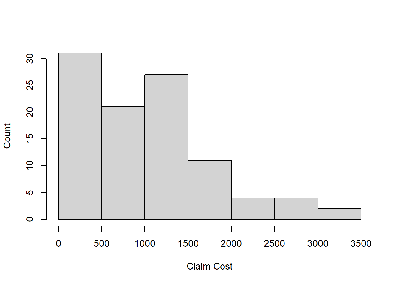
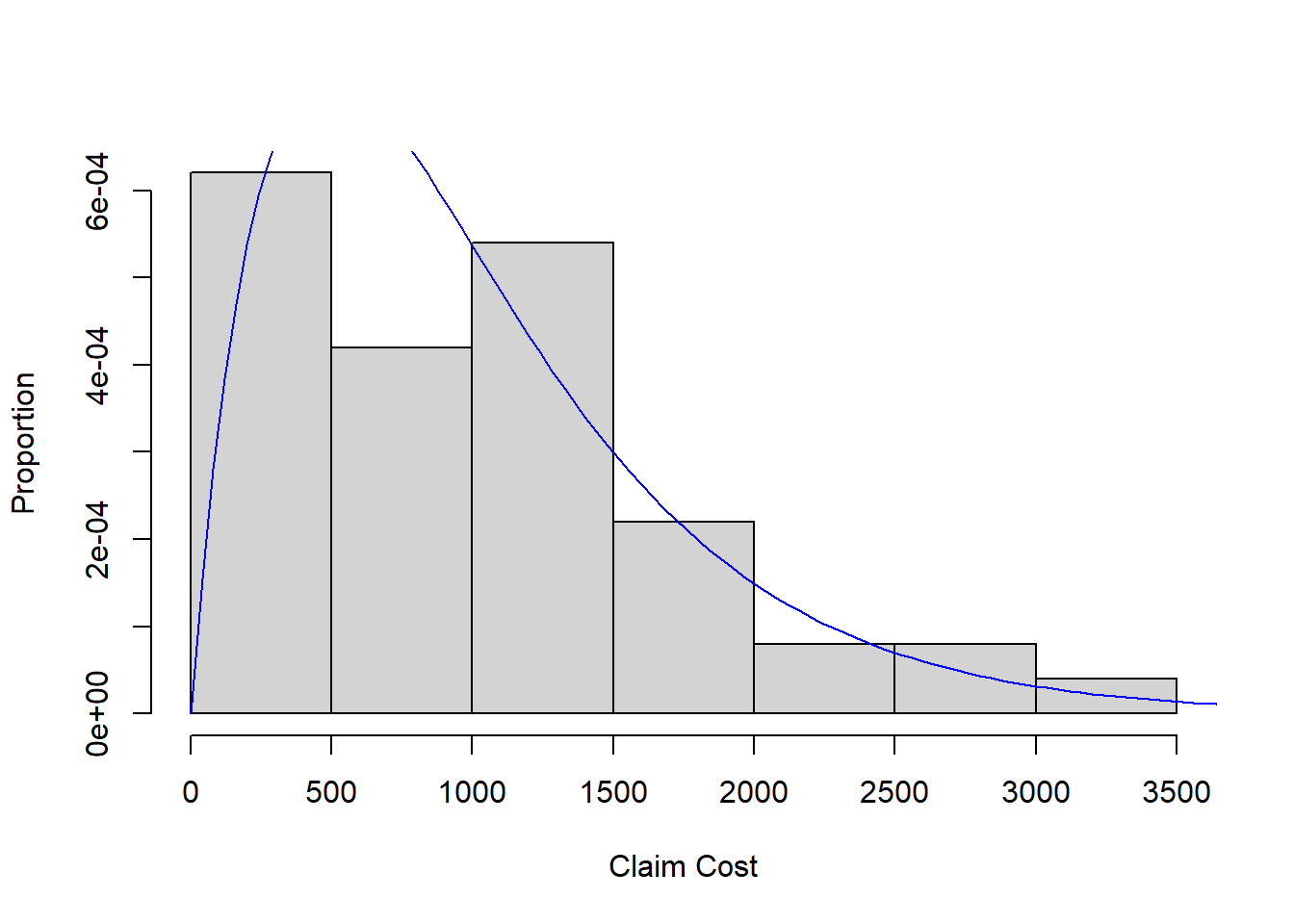
Given the auto claims are positively skewed, we will assume a Gamma distribution reasonably models the population and fit a Gamma to the data by maximum likelihood.

The Gamma density has form $$f(x;\alpha, \beta) = \frac{\beta^\alpha}{\Gamma(\alpha)}x^{\alpha-1}e^{-x\beta}, \quad x,\alpha, \beta>0$$ where $(\alpha, \beta)$ are shape and rate parameters. The likelihood for a random sample of size $n$ is $$L(\alpha, \beta; X_1, \ldots, X_n) = \left(\frac{\beta^\alpha}{\Gamma(\alpha)}\right)^n \prod_{i=1}^n (x_i)^{\alpha - 1} e^{-\beta\sum_{i=1}^n x_i}.$$ Taking the log, we have the loglikelihood function (suppressing dependence on data) $$\ell(\alpha, \beta) = n\alpha\log \beta - n\log \Gamma(\alpha) + (\alpha - 1)\sum_{i=1}^n \log(x_i) - \beta\sum_{i=1}^n x_i.$$ Next, we need the gradient (the first derivatives) w.r.t. the parameters $(\alpha,\beta)$: $$\frac{\partial \ell}{\partial \alpha} = n\log\beta - \text{DiGamma}(\alpha) + \sum_{i=1}^n \log(x_i)$$ where the function DiGamma$(\alpha)$ is the logarithmic derivative of the Gamma function. Next, we have $$\frac{\partial \ell}{\partial \beta} = \frac{n\alpha}{\beta} - \sum_{i=1}^n x_i.$$

We also need the second derivatives in order to compute the Fisher information: $$\frac{\partial^2 \ell}{\partial \alpha^2} = -\text{TriGamma}(\alpha)$$ where the TriGamma function is (you guessed it!) the second logarithmic derivative fo the Gamma function $\Gamma(\alpha)$.
$$\frac{\partial^2 \ell}{\partial \alpha\partial\beta} = n/\beta.$$ $$\frac{\partial^2 \ell}{\partial \beta^2} = -\frac{n\alpha}{\beta^2}.$$

You may have guessed we will not be able to compute the MLEs by hand by solving $\frac{\partial \ell}{\partial \alpha}=0$ and $\frac{\partial \ell}{\partial \beta} = 0$. Instead, we need an iterative solver (an algorithm). In R we can use optim to solve for the MLEs. Or, we can code our own version of Newton’s method…

n <- length(data)
loglik <- function(param){
  sum(dgamma(data, shape = param[1], rate = param[2], log = TRUE))
}
grad <- function(param){
  g1 <- n*log(param[2]) - n*digamma(param[1]) + sum(log(data))
  g2 <- n*param[1]/param[2] - sum(data)
  return(c(g1,g2))
}
H <- function(param){
  h1 <- -n*trigamma(param[1])
  h2 <- n/param[2]
  h3 <- -n*param[1]/(param[2]^2)
  return(matrix(c(h1,h2,h2,h3),2,2))
}

m <- mean(data)
v <- var(data)

beta0 <- m/v
alpha0 <- m*beta0

delta <- 0.00001
diff.step <- 1
par.old <- c(alpha0, beta0)
steps <- 0
while((diff.step > delta) & (steps < 100)){
  par.new <- par.old - solve(H(par.old))%*%matrix(grad(par.old),2,1) 
  diff.step <- max(abs(par.new - par.old))
  steps <- steps + 1
  par.old <- par.new
}
par.old

##             [,1]
## [1,] 1.966640491
## [2,] 0.001948425

loglik(par.old)

## [1] -780.5969

H(par.old)

##             [,1]         [,2]
## [1,]   -65.86955     51323.52
## [2,] 51323.51588 -51803341.74

solve(H(par.old))

##               [,1]          [,2]
## [1,] -6.657160e-02 -6.595499e-05
## [2,] -6.595499e-05 -8.464786e-08

mle.optim <- optim(c(alpha0, beta0), loglik, gr = grad, control = list(fnscale = -1), method = 'BFGS', hessian = TRUE)

## Warning in dgamma(data, shape = param[1], rate = param[2], log = TRUE): NaNs
## produced

## Warning in dgamma(data, shape = param[1], rate = param[2], log = TRUE): NaNs
## produced

## Warning in dgamma(data, shape = param[1], rate = param[2], log = TRUE): NaNs
## produced

## Warning in dgamma(data, shape = param[1], rate = param[2], log = TRUE): NaNs
## produced

## Warning in dgamma(data, shape = param[1], rate = param[2], log = TRUE): NaNs
## produced

## Warning in dgamma(data, shape = param[1], rate = param[2], log = TRUE): NaNs
## produced

## Warning in dgamma(data, shape = param[1], rate = param[2], log = TRUE): NaNs
## produced

## Warning in dgamma(data, shape = param[1], rate = param[2], log = TRUE): NaNs
## produced

## Warning in dgamma(data, shape = param[1], rate = param[2], log = TRUE): NaNs
## produced

## Warning in dgamma(data, shape = param[1], rate = param[2], log = TRUE): NaNs
## produced

## Warning in dgamma(data, shape = param[1], rate = param[2], log = TRUE): NaNs
## produced

## Warning in dgamma(data, shape = param[1], rate = param[2], log = TRUE): NaNs
## produced

## Warning in dgamma(data, shape = param[1], rate = param[2], log = TRUE): NaNs
## produced

mle.optim

## $par
## [1] 1.966641732 0.001948426
## 
## $value
## [1] -780.5969
## 
## $counts
## function gradient 
##       34        4 
## 
## $convergence
## [1] 0
## 
## $message
## NULL
## 
## $hessian
##             [,1]         [,2]
## [1,]   -65.86951     54017.32
## [2,] 54017.31581 -70328540.92

solve(mle.optim$hessian)

##               [,1]          [,2]
## [1,] -4.101660e-02 -3.150366e-05
## [2,] -3.150366e-05 -3.841603e-08