4 The geometric Brownian motion model of asset value and Monte Carlo simulation

4.1 Asset values as random variables

Let $\{S_t, t\geq 0\}$ denote the values of an asset at times $t$. Ideally, we think of time as a continuum, so that $S_t$ is a continuous process. Practically, however, we will approximate the continuous process by a discrete one by performing computations associated with the process at a grid of $t$ values in some interval $[0,T]$ with mesh-size $\Delta t$.

We model the process $S_t$ as a random or stochastic sequence; essentially, it is just a sequence of realizations of random variables.

Here is a plot of Apple’s (AAPL) close-of-day stock price and logarithm of return $\log(S_t/S_{t-1})$ from its initial listing to the present day. Stock prices are available much more often than daily, so the data visualized below already represent a discretization of the underlying process (with mesh-size 1 day).

import numpy as np
import numpy.random as npr
import matplotlib as mpl
from matplotlib.pylab import plt 
import math

plt.style.use('seaborn')
mpl.rcParams['font.family'] = 'serif'

import pandas as pd
import yfinance as yf
from yahoofinancials import YahooFinancials

aapl_df = yf.download('AAPL')

## 
[*********************100%***********************]  1 of 1 completed

close_price = aapl_df['Adj Close']
log_rets = np.log(close_price / close_price.shift(1))
aapl_df['log_rets'] = log_rets
aapl_df[['Adj Close', 'log_rets']].plot(subplots=True, figsize=(10, 6))

## array([<AxesSubplot:xlabel='Date'>, <AxesSubplot:xlabel='Date'>],
##       dtype=object)

plt.show();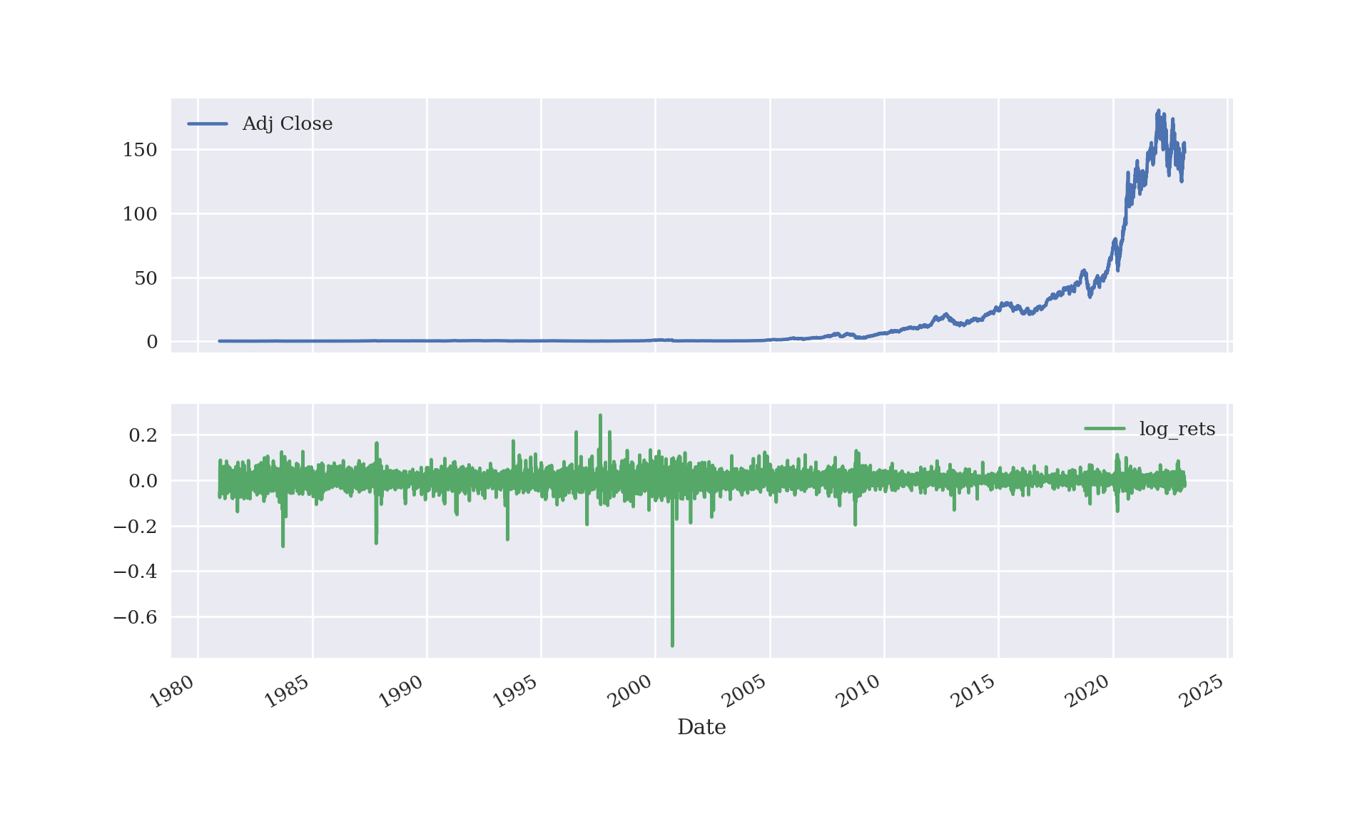

4.2 Geometric Brownian motion model of asset prices over time

The mathematics of continuous stochastic processes is advanced. Rather than presenting a full account here we focus on an intermediate level of understanding of one of the most common models used for asset prices. Later we will modify the model to account for several real-life phenomena.

It is folk-wisdom that the log returns of at asset $\log\frac{S_t}{S_{t-1}}$ are normally-distributed, or, rather, are modeled as such. This comes as a consequence of modeling the sequence of asset prices as a geometric Brownian motion.

A Brownian motion (which is also called a Wiener process) is essentially a sequence of normal random variables. Specifically, the process $W_t$ satisfies - $W_0 = 0$ - $W_t$ is continuous a.s. - $W_t$ has independent increments - $W_t - W_s \sim N(0,t-s)$ for $0\leq s\leq t$ Additionally, the sequence is measurable with respect to a filtration, an ordered family of sigma-fields (for details see, for example, Resnick’s A Probability Path Chapter 10).

The geometric Brownian motion (gBm) model says changes in asset price from time $t$ to time $t+s$ are determined by a Brownian motion and a drift. This is typically written in the following fashion as a stochastic differential equation (SDE) with respect to instantaneous price change: $$dS_t = rS_tdt + \sigma S_t dW_t$$ where $r$ is a risk-free interest rate, $dt$ is an instantaneous change in time, $\sigma$ is a volatility (standard deviation) parameter, and $W_t$ is a Brownian motion.

It is important to keep in mind the SDE doesn’t really mean anything—rather, it is simply notation used to express a stochastic integral in a concise manner. A more meaningful expression of the geometric Brownian motion model is given by the difference equation $$S_{t+s} = S_t = \int_t^{t+s} rS_u\,du + \int_{t}^{t+s} \sigma S_u \, dW_u.$$ The primary challenge to overcome is how to define integration with respect to the Brownian motion $W_u$. For various technical reasons, such an integration cannot behave exactly in the same way integration works for real-valued functions, i.e., Riemann integration. A new theory of integration, Ito integration, is needed.

Rather than giving a thorough treatment of Ito’s calculus, we will simply provide an informal derivation of Ito’s Lemma, which is enough to provide a solution” to the geometric Brownian motion. Let $f(t,\,S_t)$ be a function of time and asset price at time $t$. Take a two term Taylor expansion of $f$ and use the geometric Brownian motion SDE in the chain rule as follows:

$$\begin{align*} df &= \frac{\partial f}{\partial t}dt + \frac{\partial f}{\partial S_t}dS_t + \frac{1}{2}\frac{\partial^2 f}{\partial S_t^2}dS_t^2 + \cdots\\ & = \frac{\partial f}{\partial t}dt + \frac{\partial f}{\partial S_t}(rS_tdt + \sigma S_t dW_t) + \frac{1}{2}\frac{\partial^2 f}{\partial S_t^2}(r^2S_t^2dt^2 + 2r\sigma S_t^2 dtdW_t + \sigma^2S_t^2dW_t^2) + \cdots. \end{align*}$$

Then, Ito’s Lemma says $dW_t^2 = O(dt)$ and the substitution $dW_t^2 = dt$ is justified, while the terms $dt^2$ and $dt\,dW_t$ are ignorable and may be substituted by zero. The Taylor expansion simplifies, according to Ito, to $$df = \left(\frac{\partial f}{\partial t} + r S_t\frac{\partial f}{\partial S_t} +\frac{\sigma^2}{2}S_t^2\frac{\partial^2 f}{\partial S_t^2}\right)dt + \sigma\frac{\partial f}{\partial S_t}S_t \,dW_t.$$

Now, let $f(t,\, S_t):= \log(S_t)$, the log asset price at time $t$. In that case, we have the following derivatives: $$\partial f/\partial t = 0\quad \partial f/\partial S_t = 1/S_t \quad \partial^2 f/\partial S_t^2 = -1/S_t^2.$$ Substituting these into the SDE above, we get $$d\log S_t = r\,dt - \frac{\sigma^2}{2S_t^2}S_t^2\,dt + \frac{\sigma}{S_t}S_t\,dW_t.$$ Next integrate both sides: $$\log S_t = \log(S_0) + \left(r - \frac{\sigma^2}{2}\right)t + \sigma\, W_t.$$ Exponentiate to obtain
$$S_t = S_0\exp\left(rt - \frac{\sigma^2}{2}t+\sigma \, W_t\right).$$ Recall that $W_t - W_0 := W_t$ has variance $t$ and see that $S_t/S_0$ is log-normally distributed with parameters $(r - \sigma^2/2)t$ and $\sigma\, t^{1/2}$, which means it is right-skewed with mean $\exp(rt)$ and variance $(\exp(\sigma^2 t)-1)\cdot\exp(2rt)$.

Armed with Ito’s Lemma, we have confirmed the folk-wisdom that log-returns from time $t$ to $t+s$ are (modeled as) normal random variables with mean $(r - \frac{\sigma^2}{2}) s$ and variance $\sigma^2 s$. One last minor point: if $S_t/S_0$ has a lognormal distribution with density $f$, then the density of $S_t$ is simply $$g(s) = S_0^{-1}f(s/S_0),$$ a scaled log-normal. This is helpful, e.g., for comparing the exact distribution of $S_t$ to MC samples values of $S_t$, as we do below.

4.3 Monte Carlo simulation of the gBm model

As we showed above, there is an exact solution to the geometric Brownian motion SDE—namely, a continuous time random process characterized by independent, normal log-returns over disjoint time periods. Equivalently, given the asset value $S_0$ at time zero we know $S_t/S_0$ is log-normally distributed with the parameters given above.

Later, we will modify (complicate) the gBm model to take into account several real-life phenomena including, e.g., time-varying volatility. The augmented models do not necessarily have explicit solutions like the gBm model. Alternatively, we can simulate many times from the model to compute approximate solutions—this is called Monte Carlo. It’s not needed for the gBm model, but we will illustrate it here in order to take advantage of the simplified setting of gBm before moving on to more complicated models.

Below we compare three methods for computing $S_T$ at time $T$, given $S_0$, $\sigma$, and $r$: the explicit solution due to Ito, a Monte Carlo (MC) simulation from the lognormal distribution, and a MC simulation of paths of asset values $S_s$ for a discretization $s\in \{s_0 = 0, s_1, \ldots, s_{M+1} = T\}$. All three provide the same answer (in a distributional sense) but the MC procedures contain some additional MC variability (noise) that decreases as the number of simulations increases.

import numpy as np
import numpy.random as npr
import matplotlib as mpl
from matplotlib.pylab import plt 
import math
from scipy.stats import lognorm
plt.style.use('seaborn')
mpl.rcParams['font.family'] = 'serif'


S0 = 100
r = 0.05
sigma = 0.25
T = 2.0

# Exact density of ST based on gBm model
mu = np.exp((r - sigma**2/2)*T)
s = sigma * math.sqrt(T)
x = np.linspace(lognorm.ppf(0.001, s, scale = mu), lognorm.ppf(0.999, s, scale = mu), 1000)


# MC sampling of density of ST
I=10000
ST = S0 * np.exp((r-0.5*sigma**2)*T + sigma*math.sqrt(T)*npr.standard_normal(I))


# MC sampling of asset price path S0 to ST at 50 equally-spaced timepoints
M=50
dt = T / M
S = np.zeros((M+1, I))
S[0] = S0
for t in range(1,M+1):
    S[t]=S[t-1]*np.exp((r - 0.5*sigma**2)*dt + sigma*math.sqrt(dt)*npr.standard_normal(I))


# Plots of asset Price distribution at T = 2
plt.figure(figsize = (10,6))
plt.subplot(211)
# histogram of MC samples from scaled log-normal
hist1 = plt.hist(ST,100,density = True)
# scaled log-normal density
dens = plt.plot(x*S0, (1/S0)*lognorm.pdf(x, s, scale = mu),
       'r-', lw=2, alpha=0.6)
plt.ylabel('Asset Price')
plt.title('Exact and MC-simulated Asset Price at Time T=2')
plt.xlim([0,400])
#plt.ylim([0,0.0014])

## (0.0, 400.0)

plt.subplot(212)
# histogram of path-wise MC samples from scaled log-normal over grid of 50 times
hist2 = plt.hist(S[-1],100,density = True)
dens = plt.plot(x*S0, (1/S0)*lognorm.pdf(x, s, scale = mu),
       'r-', lw=2, alpha=0.6)
plt.ylabel('Asset Price')
plt.xlabel('Time')
plt.xlim([0,400])
#plt.ylim([0,0.0014])

## (0.0, 400.0)

plt.show()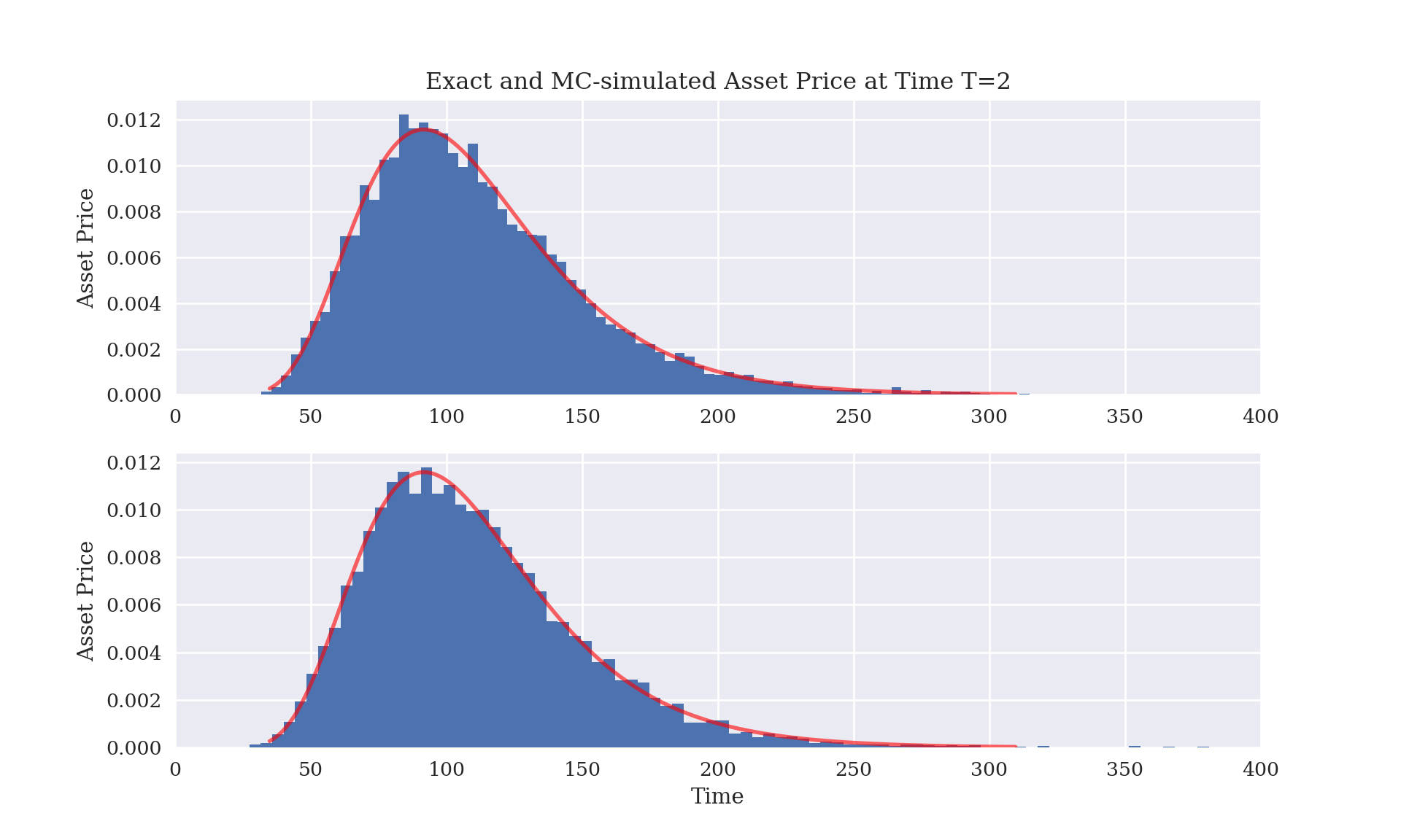

4.4 Off on a tangent: reducing MC variability

The difference between the theoretic (exact) values for the mean and standard deviation of $S_T$ and the corresponding MC approximations (shown below) is due to MC error. The Law of Large Numbers (LLN) implies MC error declines to zero as the number of MC samples increases to infinity. In practice, using many more MC samples in order to reduce MC error has the trade-off of increasing computation time (and memory usage if storing those random variates in a vector). On the other hand, there are a few ways to reduce MC error by making more clever choices of MC samples.

import scipy.stats  as scs

def print_stats(a2,a3):
    stat2 = scs.describe(a2)
    stat3 = scs.describe(a3)
    print('%14s %14s %14s %14s' % ('statistic', 'data set 1', 'data set 2', 'data set 3'))
    print(45 * '-')
    print('%14s %14s %14.3f %14.3f' % ('size', 'NA', stat2[0], stat3[0]))
    print('%14s %14s %14.3f %14.3f' % ('min', 'NA', stat2[1][0], stat3[1][0] ))
    print('%14s %14s %14.3f %14.3f' % ('max', 'NA', stat2[1][1], stat3[1][1]))
    print('%14s %14.3f %14.3f %14.3f' % ('mean', S0*math.exp(r*T), stat2[2], stat3[2]))
    print('%14s %14.3f %14.3f %14.3f' % ('stdev', S0*math.sqrt((math.exp(sigma**2 * T)-1)*math.exp(2*r*T)), np.sqrt(stat2[3]), np.sqrt(stat3[3])))


print_stats(ST, S[-1])

##      statistic     data set 1     data set 2     data set 3
## ---------------------------------------------
##           size             NA      10000.000      10000.000
##            min             NA         28.097         27.338
##            max             NA        390.870        448.195
##           mean        110.517        110.759        110.511
##          stdev         40.327         40.583         40.726

The simplest way to reduce MC variability (besides increasing the number of samples) is to use anti-thetical variates. When sampling standard normal random variates this amounts to sampling $z$ and using both $(z,-z)$ as samples. To get $2I$ samples one only needs to actually compute $I$ samples, the remaining $I$ are the same in magnitude but with the opposite signs. This accomplishes exact mean-matching, i.e., $(2I)^{-1}\sum_{i=1}^{2I} z_i = 0$, exactly the standard normal distribution mean.

Another method for reducing MC variability is second-moment matching. Suppose we generate antithetical samples $z = (z_1, \ldots, z_I)$. Let $z^\star_i := z_i / s_{z}$ for $i=1, \ldots, I$ where $s_z$ is the sample standard deviation of $z$. Now, $z^\star$ has sample mean exactly zero and sample standard deviation exactly $1$.

Further, a Box-Cox transformation may be used if the samples $z$ have positive skew. (If they have negative skew, then the samples may be reflected about the maximum value to produce a set of positively-skewed values starting from zero.) After applying the Box-cox transformation, the resulting values $y$ should be close to symmetric (closer to a normal distribution than the original variates) and a further standardization $z^\star_i = (y_i - \overline y)/s_y$ may be used to transform the values to approximately standard normal.

The following simulation supports the use of standardized antithetic variates. By design, these had exactly zero mean and unit variance, but were slightly more likely to be skewed compared to vanilly MC samples. Box-Cox transformed variates did not perform better, and were more likely to display excess kurtosis than even vanilla MC variates. It is worth pointing out that antithetic variates may be produced sequentially while standardized variates requires storing all variates in memory, which may be a problem in some applications.

import scipy.stats  as scs
import numpy  as np
import numpy.random  as npr

def bc_standardize(z):
  M = np.max(z)
  zM = M-z+0.0000001
  y = scs.boxcox(zM)
  m = np.mean(y[0])
  s = np.std(y[0], ddof=1)
  z_star = (y[0]-m)/s
  return z_star

def at_standardize(z):
  s = np.std(z, ddof=1)
  z_star = z/s
  return z_star

kurtosis_vals = np.zeros((1000,8))
skew_vals = np.zeros_like(kurtosis_vals)
mean_vals = np.zeros_like(kurtosis_vals)
std_vals = np.zeros_like(kurtosis_vals)

def print_stats2():
  for i in range(1,1001):
    X = npr.standard_normal(10000)
    Z1 = npr.standard_normal(5000)
    Z2 = npr.standard_normal(5000)
    Z3 = -Z1
    Z4 = -Z2
    Z = np.concatenate((Z1,Z2))
    Y = np.concatenate((Z1,Z3))
    W = np.concatenate((Z2,Z4))
    Ystar = bc_standardize(Y)
    Wstar = bc_standardize(W)
    Yst = at_standardize(Y)
    Wst = at_standardize(W)
    stat1 = scs.describe(X, ddof = 1)
    stat2 = scs.describe(Z, ddof = 1)
    stat3 = scs.describe(Y, ddof = 1)
    stat4 = scs.describe(W, ddof = 1)
    stat5 = scs.describe(Ystar, ddof = 1)
    stat6 = scs.describe(Wstar, ddof = 1)
    stat7 = scs.describe(Yst, ddof = 1)
    stat8 = scs.describe(Wst, ddof = 1)
    mean_vals[i-1,:] = np.array([stat1[2], stat2[2], stat3[2], stat4[2], stat5[2], stat6[2], stat7[2], stat8[2]])
    std_vals[i-1,:] = np.array([stat1[3], stat2[3], stat3[3], stat4[3], stat5[3], stat6[3], stat7[3], stat8[3]])
    kurtosis_vals[i-1,:] = np.array([stat1[4], stat2[4], stat3[4], stat4[4], stat5[4], stat6[4], stat7[4], stat8[4]])
    skew_vals[i-1,:] = np.array([stat1[5], stat2[5], stat3[5], stat4[5], stat5[5], stat6[5], stat7[5], stat8[5]])

  print('%14s %14s %14s %14s %14s %14s %14s %14s %14s' % ('statistic', 'data set 1', 'data set 2', 'data set 3', 'data set 4', 'data set 5', 'data set 6', 'data set 7', 'data set 8'))
  print('%14s %14.3f %14.3f %14.3f %14.3f %14.3f %14.3f %14.3f %14.3f' % ('mean mean', np.mean(mean_vals[:,0]), np.mean(mean_vals[:,1]), np.mean(mean_vals[:,2]), np.mean(mean_vals[:,3]), np.mean(mean_vals[:,4]), np.mean(mean_vals[:,5]), np.mean(mean_vals[:,6]), np.mean(mean_vals[:,7])))
  print('%14s %14.3f %14.3f %14.3f %14.3f %14.3f %14.3f %14.3f %14.3f' % ('std mean', np.std(mean_vals[:,0]), np.std(mean_vals[:,1]), np.std(mean_vals[:,2]), np.std(mean_vals[:,3]), np.std(mean_vals[:,4]), np.std(mean_vals[:,5]), np.std(mean_vals[:,6]), np.std(mean_vals[:,7])))
  print('%14s %14.3f %14.3f %14.3f %14.3f %14.3f %14.3f %14.3f %14.3f' % ('mean std', np.mean(std_vals[:,0]), np.mean(std_vals[:,1]), np.mean(std_vals[:,2]), np.mean(std_vals[:,3]), np.mean(std_vals[:,4]), np.mean(std_vals[:,5]), np.mean(std_vals[:,6]), np.mean(std_vals[:,7])))
  print('%14s %14.3f %14.3f %14.3f %14.3f %14.3f %14.3f %14.3f %14.3f' % ('std std', np.std(std_vals[:,0]), np.std(std_vals[:,1]), np.std(std_vals[:,2]), np.std(std_vals[:,3]), np.std(std_vals[:,4]), np.std(std_vals[:,5]), np.std(std_vals[:,6]), np.std(std_vals[:,7])))
  print('%14s %14.3f %14.3f %14.3f %14.3f %14.3f %14.3f %14.3f %14.3f' % ('mean kurtosis', np.mean(kurtosis_vals[:,0]), np.mean(kurtosis_vals[:,1]), np.mean(kurtosis_vals[:,2]), np.mean(kurtosis_vals[:,3]), np.mean(kurtosis_vals[:,4]), np.mean(kurtosis_vals[:,5]), np.mean(kurtosis_vals[:,6]), np.mean(kurtosis_vals[:,7])))
  print('%14s %14.3f %14.3f %14.3f %14.3f %14.3f %14.3f %14.3f %14.3f' % ('std kurtosis', np.std(kurtosis_vals[:,0]), np.std(kurtosis_vals[:,1]), np.std(kurtosis_vals[:,2]), np.std(kurtosis_vals[:,3]), np.std(kurtosis_vals[:,4]), np.std(kurtosis_vals[:,5]), np.std(kurtosis_vals[:,6]), np.std(kurtosis_vals[:,7])))
  print('%14s %14.3f %14.3f %14.3f %14.3f %14.3f %14.3f %14.3f %14.3f' % ('mean skew', np.mean(skew_vals[:,0]), np.mean(skew_vals[:,1]), np.mean(skew_vals[:,2]), np.mean(skew_vals[:,3]), np.mean(skew_vals[:,4]), np.mean(skew_vals[:,5]), np.mean(skew_vals[:,6]), np.mean(skew_vals[:,7])))
  print('%14s %14.3f %14.3f %14.3f %14.3f %14.3f %14.3f %14.3f %14.3f' % ('std skew', np.std(skew_vals[:,0]), np.std(skew_vals[:,1]), np.std(skew_vals[:,2]), np.std(skew_vals[:,3]), np.std(skew_vals[:,4]), np.std(skew_vals[:,5]), np.std(skew_vals[:,6]), np.std(skew_vals[:,7])))
  
print_stats2()  

##      statistic     data set 1     data set 2     data set 3     data set 4     data set 5     data set 6     data set 7     data set 8
##      mean mean          0.000         -0.000         -0.000          0.000         -0.000          0.000         -0.000          0.000
##       std mean          0.010          0.010          0.000          0.000          0.000          0.000          0.000          0.000
##       mean std          0.998          1.000          1.001          1.000          1.000          1.000          1.000          1.000
##        std std          0.014          0.014          0.020          0.020          0.000          0.000          0.000          0.000
##  mean kurtosis         -0.000         -0.001         -0.000         -0.000         -0.010         -0.010         -0.000          0.000
##   std kurtosis          0.025          0.023          0.000          0.000          0.006          0.007          0.000          0.000
##      mean skew         -0.001         -0.001         -0.002         -0.002          0.002          0.003         -0.002         -0.002
##       std skew          0.048          0.047          0.066          0.069          0.063          0.067          0.066          0.069